Test Pumping Playbook

Flussdiagrammknoten

• Collate field notes

• Cleanse data and apply corrections (baro, temp)

• Graph: elapsed time, displacement, flow rate, activity

• Plot hydrograph and annotate

• Establish likely conceptual flow model

• Download and view logger data

• Obtain all required bore and aquifer input data

• Check units and conversions

• Review published T & S

• Set up file for analytic model

• Use software wizard and review tutorials

• Plot data and perform Diagnotics

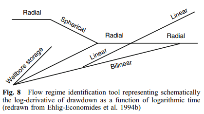
• Check derivative curve catalog

• Review log-log and semi-log 

• Capture (binary/octet-stream)

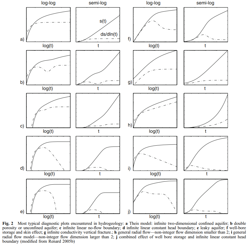
• Flat derivative indicates IARF and validity of C-J straight line

• Does flow model fit with geology?

• Choose appropriate solution

• Compare with other solutions and expected values

• Perform sensitivity analysis on T & S, Kv/Kh

• Are analysis assumptions valid?

• Use C-J semi-log straight line on late-time data when IARF

• Check Aqtesolve course notes

• Check for d-d curve inflections

• Residual d-d late time is near graph origin (reverse plot)

• Logan (confined) T=1.22.Qmax/smax

• Logan (unconfined) T=2.43.Qmax.bsat/(smax.(2b-s))

• Unconfined aquifer S=Sy (0.1-0.3)

• Specific Capacity=Q/s (m3/d/m)

• Skin Factor Sw= Aquifer Loss: BQ  Well Loss: CQ

• Batu-Driscoll (unconfined) T=1.042(Qmax/smax)

• Batu-Driscoll (confined)  T=1.385(Qmax/smax)

• Screen over water table: Semilog plot inflection. Fit later data

• Early straight line unit slope of both plots on log/log = well bore storage dominant

• If derivative does not plateau then don't use straight-line analysis

• Capture2 (binary/octet-stream)

• Early Data: bore storage Mid Data: flow model ID Late Data: boundaries

• Model-building procedure: 1.data mgt 2.diagnostics 3.model selection 4.curve matching 5.statistical analysis

• Derivative smoothing

• Deviation from unit slope as more water comes from aquifer

• log-log derivative drops to zero if leaky aquifer or constant head boundary

• The tail of derivative curve can be unreliable

• C-J gives best results for single well tests as removes skin effect

• Single well S biased by skin. Very low S = redevelop bore!

• Partial penetration gives similar curve to skin

• Theis recovery residual d-d method: t/t' intercept close to 1 = infinite aquifer. <1=no flow boundary. >1=recharge boundary

• Recovery methods:  Argawal time Theis curve match Argawal C-J plateau late time match Pap-Coop match d-d & recovery data Residual d-d Theis late time thru origin

• Perform approximation calculations

• Compare multiple values of T&S